Profile Plots#
What about the plotting the data? The next plot type down the Plots menu is ‘Profile’. By profile plots we mean an X-Y plot of any parameter versus any other parameter, with the trace for each station offset from the one before by an on-screen distance either fixed (e.g. 3 pixels apart) or proportional to the distance or relative latitude or longitude of the stations. These are sometimes called ‘waterfall’ plots. The plots are useful for oceanographic section data because physical features can be seen growing and ebbing across the section. We add an extra dimension to profile plots in Java OceanAtlas by coloring each profile by any parameter.
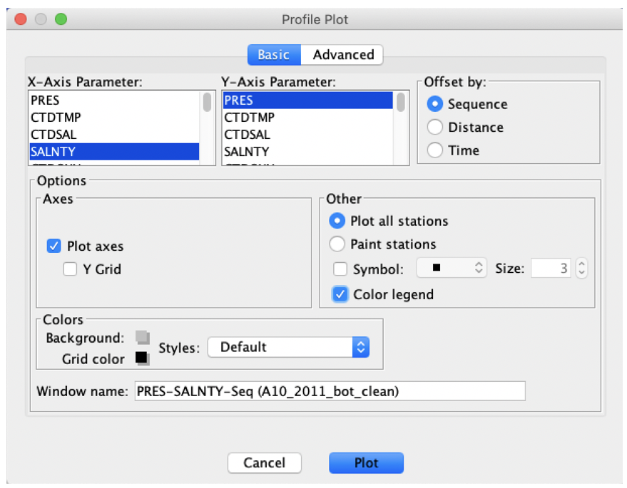
Select ‘Profile…’ from the Plots menu. Select ‘PRES’ (pressure) for the vertical (Y) axis and ‘SALNTY’ for the horizontal (X) axis, and click the ‘color legend’ box. These will be sequentially-offset plots of salinity versus pressure, the first station on the left side, each colored by a third variable. The resulting Profile Plot dialog box is shown in Fig. 4. Fig. 4 Java OceanAtlas Profile Plot dialog box, set up for a salinity (x) versus pressure (y) plot for the Atlantic A10_2011 data set.

Fig. 4 Java OceanAtlas Profile Plot dialog box, set up for the A10_2011 data.#
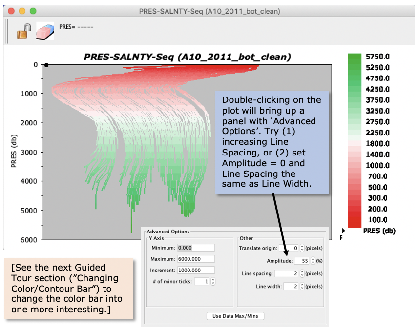
Click ‘Plot’ and the profile plot will appear, as in Fig. 5

Fig. 5 Java OceanAtlas Profile Plot from the A10_2011 data set.#
Fig. 5 shows sequential plots of salinity versus pressure, colored in accord with the color scale shown in the Data Window (should be pressure in decibars if you are using a ‘factory fresh’ copy of JOA). Try resizing the plot by click/holding on any border of the plot and dragging it to the left or right, and up and down.
Oceanographic Note
The profiles show that over most of the section the surface waters are salty, but a strong salinity minimum centered at about 750-800 decibars underlies the upper layer. Below this the water becomes much saltier, especially on the western side, but toward the bottom - at least west of the submarine ridge roughly in the middle of the section - the bottom water becomes fresher. Oceanographers know that this is subtropical surface water above Antarctic Intermediate Water above North Atlantic Deep Water above Antarctic Bottom Water. This great layering is one reason the South Atlantic sections make such good demonstration examples.
‘Decibars’? We elected to use pressure units rather than depth units in Java OceanAtlas because for most modern section data pressure is the measured parameter (from the CTD) but depth is calculated (from inverting the hydrostatic relationship PRES = ρgdz, where ρ is the density of seawater). It so happens for seawater that a pressure expressed in decibars and a depth expressed in meters are quite close numerically (roughly 1% different). So for all practical purposes a pressure of 750 decibars corresponds to a depth of about 750 meters (actually the depth in this example would be about 746 meters).
Did you notice that the Y axis in Figure 5 is reversed, i.e. it runs from the minimum value at the top to the maximum at the bottom? This makes oceanographic sense, of course, which is why oceanographers use this ‘left-handed coordinate system’ for pressure and density. The parameter headings fed into Java OceanAtlas contain an optional marker which, when present, tells the application to reverse the Y-axis, as here.
And the ‘submarine ridge roughly in the middle of the section’? Because the data from each Atlantic A10_2011 station extend to within roughly 10 meters of the bottom, the deepest portions of each profile plot line, when linked, form a rough depiction of the bathymetry underlying the section. The ridge is the great Atlantic Mid-Ocean Ridge.
The coloring of each profile by pressure is not very informative when pressure is already the Y-axis. We will next change that. [Leave the plot on the screen.]