Property-Property Plots

Oceanographic Note

Property-property plots (X-Y plots) are essential to oceanographic data interpretation. As the science of oceanography developed in the late 1800s, and as physical/chemical observations became available from widespread regions, it became apparent that ocean waters had imprinted upon them clear and traceable patterns of characteristics. For example, waters originally from the sea surface in a region of low air temperatures and high precipitation would remain relatively cold and fresh as they spread from their source region, whereas those from the subtropics remained warm and salty due to heating and evaporation there.

The most basic oceanographic property-property plot is a property plotted against pressure (or depth) as the vertical axis. However, physical oceanographers have a special fondness for temperature versus salinity plots (often as not potential temperature versus salinity plots for the reasons discussed earlier in the Guided Tour), because of the imprinting from the source regions and because isopycnals at appropriate reference pressures can be added to potential temperature versus salinity X-Y plots.

For example, we show in Fig. 9 a potential temperature versus salinity plot prepared from a global selection of data (a long section from many cruises extending from the Ross Sea to the Bering Sea in the Pacific Ocean, across the Arctic Ocean and Nordic Seas, and then from Iceland to the Weddell Sea in the Atlantic Ocean), colored by a specially-made color-contour bar with equal divisions of sigma-0 from 22.7 to 27.95.

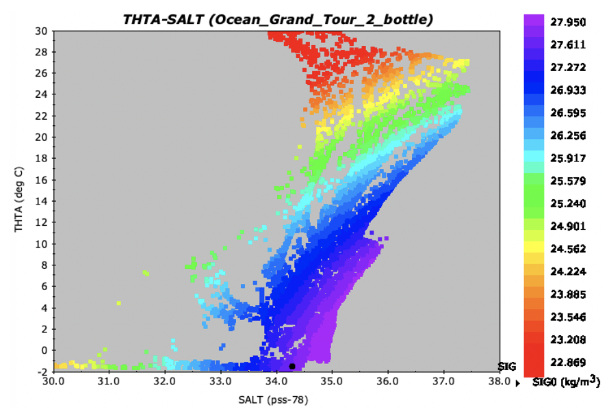
Fig. 9 Property-property plot of potential temperature versus salinity for an Antarctic-Pacific-Arctic-Atlantic-Antarctic section, with data points colored by 32 equally-spaced values of the density parameter Sigma-0.

Each transition of the bands of color in Fig. 9 marks an isopycnal. You can visualize which waters along this section would most readily mix, that is, if they were brought together.

Many property-property correlations are of interest to oceanographers. In Java OceanAtlas we permit you to plot any observed or calculated parameter versus any other, and to color the data points by any color bar which corresponds to a parameter named in the Data Window.

As noted previously in the Guided Tour, we have configured the dialog boxes for each JOA plot type so that a basic plot can be made with a minimum of user input:

For a JOA property-property (X-Y) plot, the ‘Plot’ button is activated after at least one parameter is chosen for the X-axis [up to 7 can be selected via command-clicking] and any one parameter is selected for the Y-axis. No further user actions are required other than clicking ‘Plot’.

Select ‘Property-property…’ from the ‘Plots’ menu. Set up a potential temperature-salinity plot, by selecting THTA for the Y-axis and SALNTY for the X-axis. Select ‘Color Legend’, which adds the current color bar to the plot, make the marker size ‘5’, and ‘Connect observations’, which will add a line connecting the observations at the station currently in the Data Window. Also, because this is a potential temperature versus salinity plot, we can add isopycnals - lines of constant density - to the plot (same holds for a temperature (CTDTMP) versus salinity plot): click on the ‘Advanced’ tab near the top of the dialog box, and near the bottom of the Advanced panel click on ‘Isopycnals’, leaving the ‘Pressure’ slider set to ‘0’ decibars. On the Advanced panel you can also adjust the X-axis range to 34 to 37 with an increment of 0.5 and the Y-axis range to 0 to 24 with an increment of 2. See Fig. 10 for a picture of both parts of the dialog box with these selections.

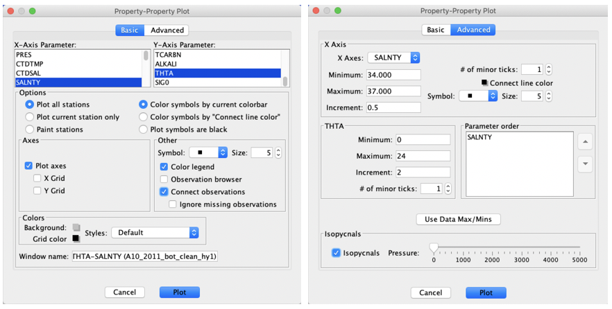
Fig. 10 Java OceanAtias Property-Property dialog box: (left) Basic panel, set up for a potential temperature (Y) versus salinity (X) plot as described in the text, and (2) the Advanced panel with axis-range changes and selection of adding isopycnals at 0 db reference pressure (sigma-0).

Click ‘Plot’ in the Property-Property Plot dialog box, and you should see the plot shown in Fig. 11.

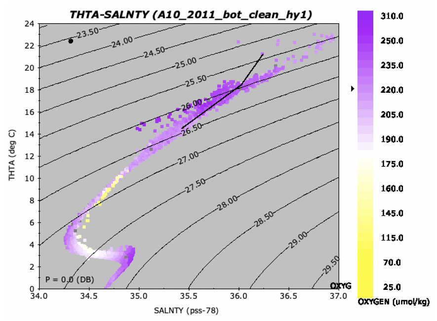
Fig. 11 Property-property plot of potential temperature versus salinity, with isopycnals, for the A10_2011 section, with data points colored by dissolved oxygen(the data dots are colored by whatever parameter is shown in the Data Window).

Now again select ‘Property-property…’ from the Plots menu. Set up a THTA (Y-axis) - SILCAT (X-axis) plot. This time, experiment with the tick-mark options by clicking on the ‘Advanced’ tab near the top of the dialog box. Set the silicate (X-axis) range from 0 to 140, with an axis increment of 20 and 3 minor ticks between each labeled axis tick, and set the potential temperature (THTA, Y-axis) increment to 5 and 4 minor ticks between each labeled axis tick. See Fig. 12 for the Property-Property Plot dialog box set up this way, and see Fig. 13 for the resulting plot.

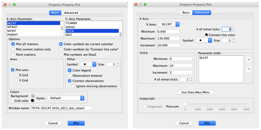
Fig. 12 Java OceanAtlas Property-Property dialog box: (left) Basic panel, set up for a potential temperature (Y) versus silicate (X) plot as described in the text, and (2) the Advanced panel with axis-range changes. Isopycnals cannot be added to any X-Y plot except a temperature (or potential temperature) versus salinity plot.

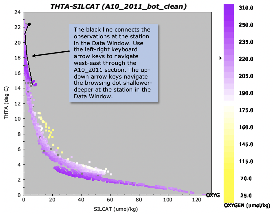
Fig. 13 Property-property plot of potential temperature versus silicate for the A10_2011 section, with data points colored by dissolved oxygen.

You now should have on your monitor screen a Data Window, a map, one ‘profile’ plot, and two ‘property-property’ plots.

Oceanographic Note

There is much that can be said about the potential temperature - salinity and potential temperature - silicate plots:

First, on the Θ-S plot, examine the values on the labeled isopycnals. The warmer or the fresher the water, the smaller the value - the less the density - and the colder or saltier the water, the higher the value - the greater the density. Less dense water always overlies more dense water, but in portions of many vertical profiles, although the density profile is stable, the influence of temperature on density opposes that of salinity, with one of the changes being stronger and thus creating a stable profile. For example, warm, salty water may lie on top of colder, fresher water if the colder, fresher water is more dense. In that case the influence of that specific temperature difference in making the deeper, colder water denser is greater than that of the salinity difference in making the deeper, fresher water less dense. This is exactly the case in the Θ-S plot of the South Atlantic A10_2011 section data. Remembering that less dense water will always lie on top of more dense water, the isopycnal labels indicate the vertical sense of the data in the Θ-S plot: warm, mostly salty tropical surface water - at some stations the surface water is fresher than at others, perhaps due to rainfall - overlies colder, fresher water known as Antarctic Intermediate Water (AAIW), with a cold/fresh AAIW extremum near about 4°C and a salinity of 34.4. The AAIW has spread northward from its source in the Antarctic Circumpolar Current zone in winter under cold air temperatures, and that zone is a region where there is ample precipitation, so it is relatively cold and fresh.

Beneath the AAIW - i.e. at densities immediately greater than that of the AAIW - the water becomes saltier, with not very much temperature change. This layer originates in the North Atlantic Ocean from a blend of cold, dense waters from the Labrador Sea and dense overflows into the North Atlantic from the Nordic Seas, and so is called North Atlantic Deep Water (NADW). The Atlantic Ocean is the saltiest of the major oceans - due in part to the influence of the Mediterranean Sea - and so its dense products tend to be salty as well.

Underneath the NADW the water again becomes colder and fresher. These abyssal waters originate as a blend of very cold, relatively fresh, dense bottom waters from the Weddell Sea with Antarctic Circumpolar Deep Water and NADW, and are known away from the Antarctic as Antarctic Bottom Water (AABW).

The perceptive observer may note something odd: In the Θ-S plot (Fig. 11) the coldest, freshest AABW appears to be very slightly ‘less dense’ than some of the water about halfway between the coldest/fresh extremum and the NADW extremum. [You can see this more clearly if you jump ahead to Extracting Selections to learn about extracting selections from plots and try it on this feature.] How can this be? The answer is simple enough, though not so easy to explain: Density of seawater is a strong function of pressure. But the effect of temperature on density is itself also a function of pressure. It is an observed fact that warmer water resists compression better than does colder water, all other factors being equal. (Imagine that the increased motion of the water molecules of the warmer water - temperature is partly a measure of the motion of molecules - enables them to better resist being compressed.) And so if you have two parcels of water at the sea surface of equal density at the sea surface, but one is warm and salty and the other is cold and fresh - the two parcels would lie along one of the isopycnal lines in Fig. 11 - but then move them adiabatically to 4000 decibars, the colder, fresher parcel will be compressed more and will then be denser (at 4000 decibars) than the warm, salty parcel. Thus to avoid confusion when comparing the densities of water samples, the densities must be compared at a pressure appropriate to the comparison. The isopycnals in Fig. 11 were calculated with a ‘reference pressure’ of 0 decibars, i.e. with respect to sea surface pressure. But the South Atlantic deep waters lie near 4000 meters, and so a reference pressure of 4000 decibars would be more nearly appropriate. Double-click on the Θ-S plot, and in the isopycnals portion of the dialog box move the ‘pressure’ slider to ‘4000’; then click ‘OK’. You will see a dramatic change in the slopes of the isopycnals, which are now drawn with respect to 4000 decibars pressure, and now it will be clear that in the deep and bottom water along the Atlantic A10 section the AABW underneath the NADW is truly more dense than the NADW, as indeed it must be. This effect of temperature on the compressibility of seawater may seem subtle, but it is a relationship crucial to physical oceanography.

There is no density implication to the potential temperature - silicate relationships (Fig. 13), but recalling that the temperature values there are of course identical in the Θ-S plot (Fig. 11), it is easy to see that the warm upper layer waters are depleted in dissolved silica, with a marked increase of silicate into the AAIW, followed by an abrupt decrease of silicate in NADW, and then a very sharp increase of silicate into the AABW, with a bottom maximum. This pattern makes good oceanographic sense: silicate is used by diatoms to make their shells, and is often depleted in the upper layers by plankton uptake. Antarctic-source waters found in the South Atlantic have a higher silicate concentration than do North Atlantic waters because silicate is cycled in great abundance in the Antarctic zone by planktonic activity, and the AAIW and AABW layers arise partly from the deeper layers where the shells from diatoms dissolve. Also, the deep Antarctic circumpolar waters receive the deep waters of the Pacific Ocean, which are very strongly enriched in dissolved nutrients by biological decay during their long passage as intermediate and deep layers in the Pacific. The North Atlantic Ocean is not so directly connected to this huge nutrient cycling machine and so has lower nutrient concentrations in general, in nearly every layer, than do the other oceans.

If you created the Θ-S and Θ-silicate plots in accord with this tutorial, then the data points on your plots are colored in accord with the dissolved oxygen concentration of those samples, as in Figures 11 and 13. The lower oxygen concentrations of much of the water from 5-15°C is caused by organic decay and a lack of local wintertime exchange of gases at the sea surface. But oxygen concentrations in the NADW, especially, are high. The Labrador Sea Water and the Nordic Sea overflows which helped to form NADW obtained their characteristics at the winter sea surface in their regions of origin, where they were cooled, and where, because cold waters have a greater capacity to hold dissolved gasses than do warm waters, they attained high concentrations of dissolved oxygen. Other factors in helping NADW maintain its high oxygen concentrations are that (1) the Nordic Sea outflows mix in the northern North Atlantic Ocean with relatively high oxygen water, and (2) the formation and spreading rate of NADW, relative to the capacity of the North Atlantic biological production to deplete its oxygen by decay of organic matter ‘raining’ into the NADW from above, is higher than is the case for the Pacific Ocean deep water (which as noted above has a strong influence on the Antarctic zone intermediate and deep waters). NADW is thus sometimes thought of as the ‘ventilator’ of the deep World Ocean.