Example 3D: Static Stability and Brunt-Väisälä Frequency

The DPO text discusses the important concept of static stability in the ocean. JOA offers several stability-related calculations. We will calculate and plot these, using the data file A16S_2005_sta085_bottle.joa.

Files that may be needed or created in this example:

• A16S_2005_sta085_bottle.joa

Exercise 3D-01: Seawater Properties - Stability

• File → Open… →A16S_2005_sta085_bottle.joa

• Calculations → Parameters…

  Set up the Parameter Calculations dialog box as follows, in particular choosing all three Buoyancy frequency parameters:

  

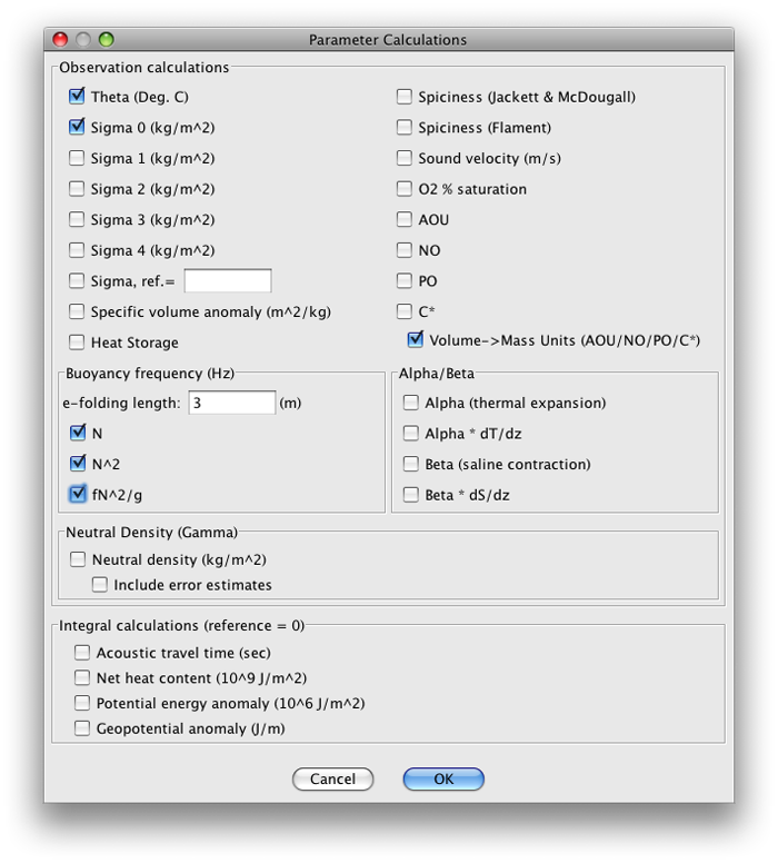
  FIG 3d-01 JOA Parameter Calculations dialog box with theta, sigma-0, and all three Bouyancy Frequency parameters checked

  The three stability-related parameters now appear in the JOA Data window:

  

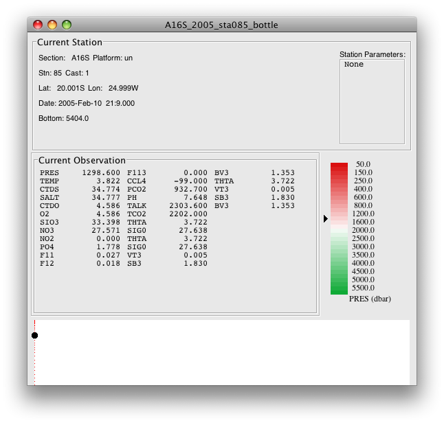
  FIG 3d-02 JOA Data Window after calculation of theta, sigma-0, and all three Buoyancy Frequency parameters

  Note

  Each time a parameter is calculated in an open JOA data file, the new calculation result is listed in the Data Window. Thus, several identical numbers for the same parameter may sometimes appear. This is normal JOA behavior and will not affect JOA plots or other actions.

• Next, set up a multiple-parameter JOA Property-Property Plot using the technique described in the earlier examples for this DPO chapter:

  To make the dialog box shown below:

  • Plots → Property-Property…

  • Now use the dialog box resizing symbol on the lower right of the dialog box to “pull down” (extend down) the dialog box (click on the symbol and move the mouse pointer down the screen). You will see the scrolling X- and Y-axis parameter lists expand until all the parameters are visible.

  • Now, via right-clicks or ctrl/command-clicks, you will find you can select more than one X-axis parameter. Do this for

    • salinity (SALT)

    • potential temperature (THTA)

    • sigma-0 (SIG0)

    • and all three buoyancy frequency related parameters (VT3, SB3, and BV3)

  • Use pressure (PRES) for the Y-axis. Also select Color symbols by “Connect line color” and Connect observations, and select square dot symbols, size 7. The Basic page of the Property-Property Plot dialog box should then look like this:

    

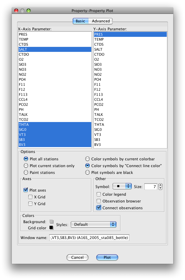
    FIG 3d-03 JOA Property-Property plot dialog box Basic panel, set up for a multi-parameter plot as described

• Now, select the Advanced panel of the Property-Property Plot dialog box.

• Customize the “Minimum” and “Maximum” values, “Increment” and “# of Minor Ticks” (and, if you wish, the “Connect line color”, “Symbol” and symbol “Size”) for each of the X-axis parameters (reached individually by scrolling through the list of X-axis parameters) and the “Minimum” and “Maximum” values, “Increment”, and “# of Minor Ticks” for the Y-axis parameter, which in this case is pressure (PRES).

  Set these up as shown in the table:

  Axis	Minimum	Maximum	Increment	# of Minor Ticks
  SALT	34	37.5	0.5	4
  THTA	0	28	2	1
  SIG0	24	28	0.5	4
  VT3	0	0.2	0.05	4
  SB3	0	50	5	4
  BV3	0	7	0.5	4
  PRES	0	6500	500	4

• Now when you click on the Plot button, you will see this plot:

  

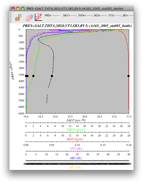
  FIG 3d-04 JOA Property-Property plot with ranges and increments as described

You may note right away that there is not much structure to stability in the deeper waters. To better visualize the portion of the water column where there is more structure:

• Return to the Advanced panel of the Property-Property dialog box:

  • Double-click or control-click on the Property-Property Plot

  • Or type [ctrl/cmd]-R or Edit → Edit: plotname when the Property-Property Plot is the front-most window

• Change the axis limits for pressure (PRES) to 0, 1200, 200, 3:

  

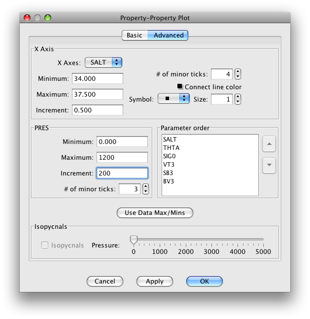
  FIG 3d-05 Detail of the Advanced panel of the JOA property-property plot dialog box

• Now when you click OK, you will see the upper 1200 decibars of the plot:

  

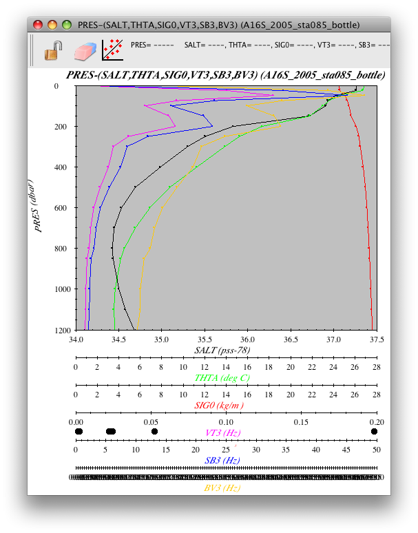
  FIG 3d-06 JOA Property-Property plot with ranges and increments as described

Examine

You can see that all three JOA stability-related parameters produce similar results with the A16S station 085 profile data, with stability maxima and minima at about the same pressures in the water column.

Later on, when you are exploring other ocean regions with JOA, you might try making similar plots to help visualize static stability there. Also, when you learn how to make vertical sections with JOA (via a later DPO JOA Example), you may find it interesting to make vertical section plots of one or more of the static stability parameters.