Example 4D: Vertical Distribution of Water Properties Along South-to-North Transects

DPO Text References:

DPO 4.7

Age of ocean water

In DPO 4.7 the concept of using ocean tracers to determine aspects of the “age” of ocean waters is discussed. We have provided a data file you can use with JOA to make an Atlantic Ocean companion to the Pacific 150°W CFC-11 section shown in DPO Figure 4.24.

Ocean CFC data are usually sparser than those averaged in the WOA05 suite of parameters (WOA05 contains vertical distributions of temperature, salinity, dissolved oxygen, silicate, nitrate, and phosphate), are sometimes noisier, and often contain more values known to be in error (so-called “bad data”, often left in data files but with a “data quality code” left in the file to indicate the value is suspect or bad).

To prepare contoured section plots, JOA interpolates the profile data onto an X-Z grid. Where grid values are missing, JOA sometimes has trouble “connecting the lines” when it draws color/contours. Hence even though we have done some cleaning of missing and bad values when we prepared the A16_2003_2005_clean_cfc.joa data file, in order to produce a pleasant-looking contour section plot with JOA, we will use some of JOA’s optional plot features. This will also provide an opportunity for you to extend your JOA section-plotting skills.

Files that may be needed or created in this example:

• A16_2003_2005_botclean_cfc.joa

Exercise 4D-01: Vertical Sections - Making a CFC Contour Plot

• Start JOA

• File → Open… → A16_2003_2005_clean_cfc.joa

• Plots → Contour…

• In the Contour Plot dialog box select F11 from the Parameter list, and PRES-0-6000_srf.xml from the Interpolation surfaces list

• Click on the Interpolations Options… button in the Contour Plot Primary Contours dialog box, and set up a far-field interpolation

  We suggest settings such as these (we show only part of the Interpolation Options dialog box here):

  

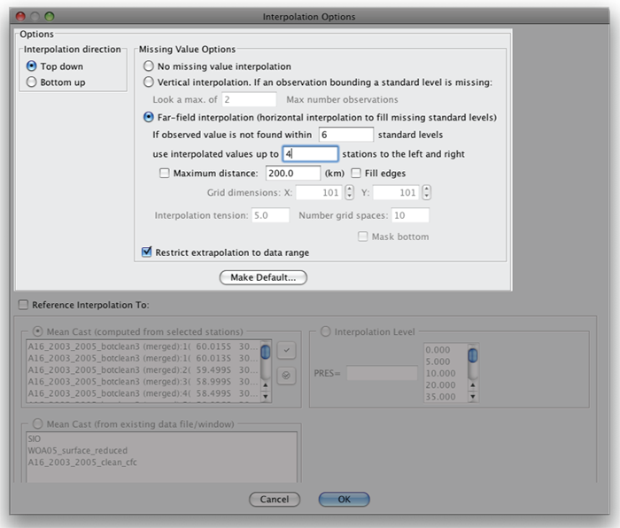
  FIG 4d-01 Interpolation Options dialog box

• Click OK in the Interpolation Options dialog box to return to the Contour Plot dialog box

• Under Colorbars: scroll through the list to see if your copy of JOA already has a color bar for F11. If it does, just select it. If not, here is how you can create an F11 colorbar on the fly:

  • In the Primary Contours window of the Contour Plot dialog box, see the Create autoscale colorbar sub-panel.

    

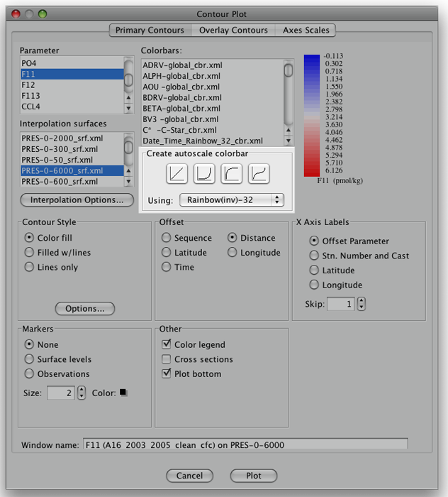
    FIG 4d-02 Create autoscale colorbar sub-panel

  • With the palette Rainbow(inv)-32 selected (see to the right of Using:) click on the left-most of the four choices of ramp for the new color bar.

    This will provide 32 contours at equal intervals of CFC-11 from the lowest value in the interpolated data set to the highest value in the interpolated data set.

    Note

    We emphasized “in the interpolated data set” to emphasize that if the interpolated data set for some reason contains values outside the upper and lower limits of the original data set - JOA might autoscale a color bar in an unrealistic way.

  • To work around this, after you have autoscaled the color bar, just double-click on the color bar, which will bring up the JOA Colorbar Editor.

  • For this CFC-oriented data set, we suggest that in the JOA Colorbar Editor you type in “0” for the Start value:, “6” for the End value:, and then click on the left-most (linear) Create with shape: ramp.

    The Colorbar Editor will then look like this:

    

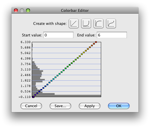
    FIG 4d-03 Colorbar Editor dialog box

  • After you click on OK in the Colorbar Editor, JOA will return you to the Contour Plot dialog box, where your new color bar will be ready to use.

• We suggest that for the other settings in the Contour Plot dialog box you set up as in this example:

  

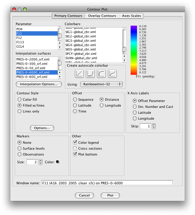
  FIG 4d-04 Primary Contour panel of the Contour Plot dialog box

• Now, when you click on the Plot button, JOA will draw this CFC-11 section:

  

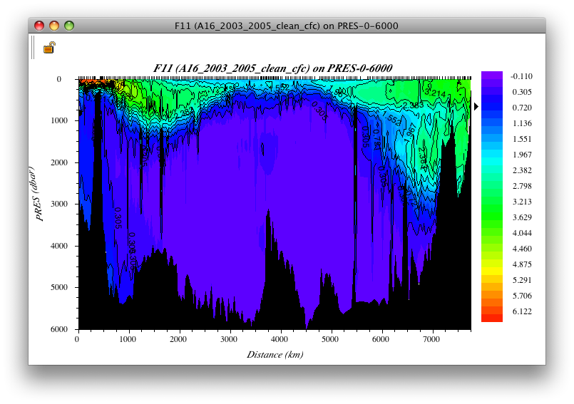
  FIG 4d-05 CFC-11 section

Examine

What are the primary differences in the CFC-11 distributions between Fig. 4.23 (Pacific Ocean) and the section drawn from the A17_2003_2005 data file?

Considering that CFCs are anthropogenic (man-made) gases that enter the oceans through dissolution at the sea surface, what might be an explanation for these Pacific versus Atlantic CFC-11 distribution differences?