Example 3E: Sound in the Sea

DPO 3.7 discusses sound in the sea. You can use JOA’s parameter calculator to calculate sound speed, and then plot the results with an eye to visualizing how sound speed varies with temperature, salinity, and pressure. Here we will use profile data at one station, the A16S_2005_sta085_bottle.joa data file.

Files that may be needed or created in this example:

• A16S_2005_sta085_bottle.joa

Exercise 3E-01: Seawater Properties - Sound Speed

• File → Open… → A16S_2005_sta085_bottle.joa

• Calculations → Parameters… Select potential temperature (Theta), density referred to sea surface pressure (Sigma 0), and Sound velocity:

  

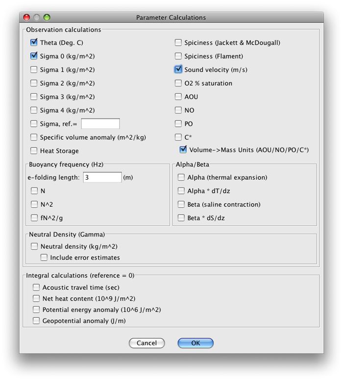
  FIG 3e-01 JOA Parameter Calculations dialog box with theta, sigma-0, and sound velocity parameters checked

• Click OK The three parameters now appear in the JOA Data window:

  

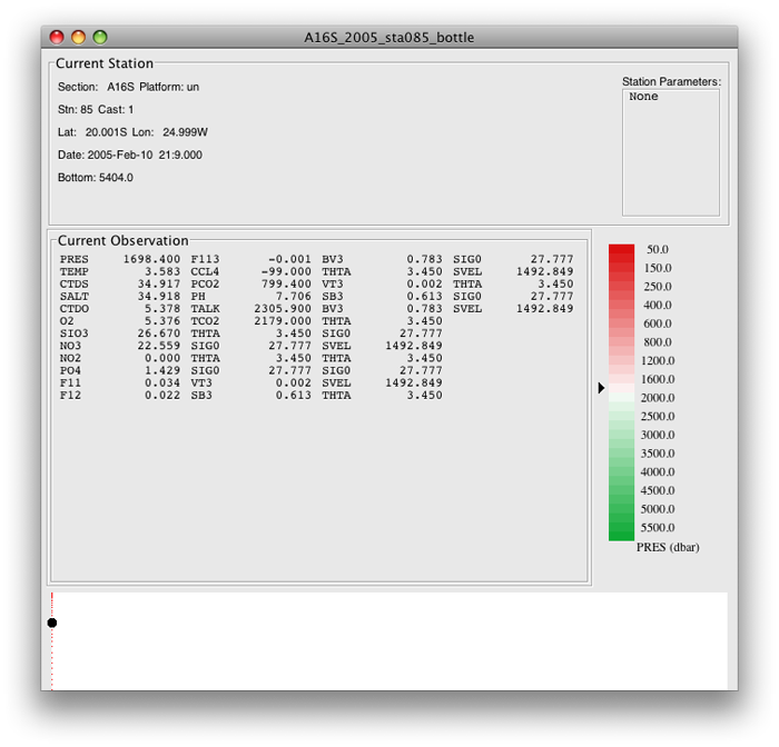
  FIG 3e-02 JOA Data Window after calculation of theta, sigma-0, and sound velocity parameters

• Next, set up a multiple-parameter JOA Property-Property Plot using the technique described in the earlier examples for this DPO chapter:

  • Plots → Property-Property…

  • Now use the dialog box resizing symbol on the lower right of the dialog box to “pull down” (extend down) the dialog box (click on the symbol and move the mouse pointer down the screen). You will see the scrolling X- and Y-axis parameter lists expand until all the parameters are visible.

  • Now, via right-clicks or ctrl/command-clicks, you will find you can select more than one X-axis parameter. Do this for salinity (SALT), potential temperature (THTA), sigma-0 (SIG0), and sound velocity (SVEL), with pressure (PRES) for the Y-axis.

  • Also select Color symbols by “Connect line color” and Connect observations, and select circular dot symbols, size 7 (to make your symbols easier to see on the resulting plot).

  The Basic page of the Property-Property Plot dialog box should then look like this:

  

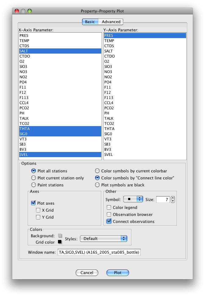
  FIG 3e-03 JOA Property-Property plot dialog box Basic panel, set up for a multi-parameter plot as described

• Property-Property Plot → Advanced As with the previous DPO JOA Example, you can now customize the “Minimum” and “Maximum” values, “Increment” and “# of Minor Ticks” (and, if you wish, the “Connect line color”, “Symbol” and symbol “Size”) for each of the X-axis parameters (reached individually by scrolling through the list of X-axis parameters) and the “Minimum” and “Maximum” values, “Increment”, and “# of Minor Ticks” for the Y-axis parameter, which in this case is pressure (PRES).

  Set these up as shown in the table:

• Set up the Advanced panel of the Property-Property Plot dialog box with these values:

  AXIS	Minimum	Maximum	Increment	# of minor ticks
  SALT	34	37.5	0.5	4
  THTA	0	28	2	3
  SIG0	24	28	0.5	4
  SVEL	1450	1600	50	4
  PRES	0	6500	500	4

• Now when you click on the Plot button, you will see this plot:

  

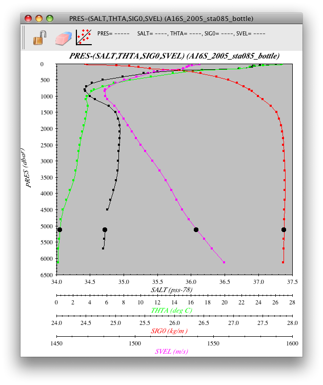
  FIG 3e-04 JOA Property-Property plot with ranges and increments as described

Later in the DPO JOA Examples, when you learn how to plot vertical section data, we strongly urge you to make a vertical section of sound speed, for example with the WOA05_A16.joa data file, which covers the length of the Atlantic Ocean from Antarctic waters to Iceland. You will find such a section makes it easy to visualize the “SOFAR channel” sound speed minimum discussed in the text.