Example 6D: Maps of Properties on Density and Other Surfaces
Maps of observed or calculated parameters on density surfaces are a central tool for examining oceanographic data. These are nearly as easy to make with this JOA plotting technique as was the map on standard pressure surfaces.
Learn More
Why maps on density surfaces are so useful to oceanographers
The amount of work required to mix two different parcels of water is proportional to their density difference. Water mixes most easily with water of the same density, so there is a clear and marked tendency for source characteristics to spread out on surfaces of constant density (isopycnals), at least away from boundaries and other regions of forcing. Thus, by examining properties on isopycnals, one can gain insight into the preferred patterns of spreading of characteristics away from sources.
Files that may be needed or created in this example:
WOA05_NorthAtlantic_square.joa
Exercise 6d-01: Other Maps - Maps on Density Surfaces
Continue from 6C-01:
Go back to the Configure Map Plot dialog box by:
Double-click on the plot surface or,
With the plot window in the foreground, type [ctrl/cmd]-R
From the Station Colors tab of the dialog box, select the Iso-surface value sub-tab, and set it up as shown below:
Under Parameter: choose O2
For Surface: use SIG0-global_srf.xml (potential density referred to sea surface pressure)
Note
JOA will calculate SIG0 automatically when you choose this interpolation surface.
Use the O2-global_cbr.xml color bar under Colors:
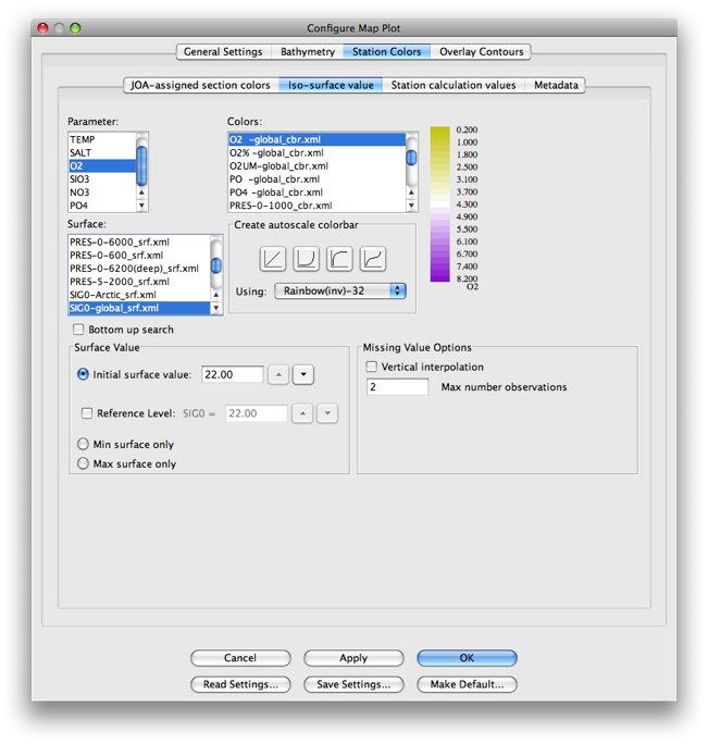
Fig 6d-01 Iso-surface sub-panel of the Station Colors panel of the Configure Map Plot dialog box
Click OK to get the map below
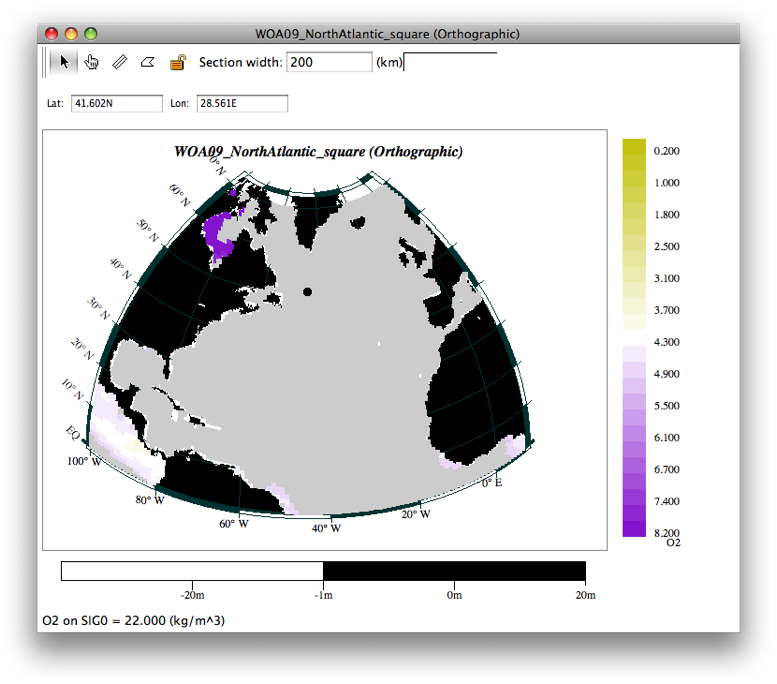
Fig 6d-02 Orthographic plot O2 on SIG0
The resulting map is much like the SALT on PRES map, but now we have O2 on SIG0, which can be browsed in the same fashion. In the image below, we have used the up and down arrow keys on the keyboard to move the active surface to SIG0 = 27.595.
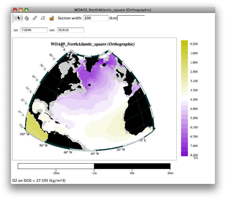
Fig 6d-03 Orthographic plot SIG0 = 27.595
Examine
The purple colors correspond to high oxygen concentrations and yellow to lows, explore this plot by keying the arrow keys up (to less dense water) and down (to more dense water). The sources of dense, high oxygen water in the Labrador Sea (between Canada and Greenland) and in the Nordic Seas (between Greenland and Norway).
You will also see evidence of the spreading of high oxygen waters from the south, and develop of areas of low oxygen in the equatorial region.